
|
Neil Lawrence ML@SITraN
|
|
|
Neil Lawrence ML@SITraN
|
Release 0.201 Fixed bug which meant that back constraint wasn't working due to failure to initialise lwork properly for dsysv. Fixed bug in gplvm.cpp which meant dynamics wasn't working properly because initialization of dynamics model learning parameter wasn't set to zero. Thanks to Gustav Henter for pointing out these problems.
In this release the dynamics model of Wang et al. has been included. The initial work was done by William V. Baxter, with modifications by me to include the unusual prior Wang suggests in his MSc thesis, scaling of the dynamics likelihood and the ability to set the signal noise ratio. A new example has been introduced for this model below.
As part of the dynamics introduction a new MATLAB toolbox for the GP-LVM has been released. This toolbox, download here, is expected to be the main development toolbox for the GP-LVM in MATLAB.
Version 0.101 was released 21st October 2005.
This release contained modifications by William V. Baxter to enable the code to work with Visual Studio 7.1.
Version 0.1, was released in late July 2005.
This was the original release of the code.
The software is written in C++ to try and get a degree of flexibility in the models that can be used without a serious performance hit. This was difficult to do in MATLAB as users who have tried version 1 (which was fast but inflexible) and version 2 (which was flexible but slow) of the MATLAB software will appreciate.
The sparsification algorithm has not been implemented in the C++ software so this software is mainly for smaller data sets (up to around a thousand points).
The software is mainly written in C++ but relies for some functions on FORTRAN code by other authors and the LAPACK and BLAS libraries.
As well as the C++ code some utilities are supplied in MATLAB code for visualising the results.
Part of the reason for using gcc is the ease of interoperability with FORTRAN. The code base makes fairly extensive use of FORTRAN so you need to have g77 installed.
The software is compiled by writing
$ make gplvm
at the command line. Architecture specific options are included in
the make.ARCHITECTURE files. Rename the file with the
relevant architecture to make.inc for it to be included.
make.atlas includes options for compiling the ATLAS
optimised versions of lapack and blas that are available on a server I
have access to. These options may vary for particular machines.
MSVC/gplvm. The compilation makes use of f2c
versions of the FORTRAN code and the C version of LAPACK/BLAS,
CLAPACK. Detailed instructions on how to compile are in the
readme.msvc file. The work to convert the code (which included ironing
out several bugs) was done by William V. Baxter. Many thanks to Bill
for allowing me to make this available.
The way the software operates is through the command line. There is
one executable, gplvm. Help can be obtained by writing
$ ./gplvm -h
which lists the commands available under the software. Help for each command can then be obtained by writing, for example,
$ ./gplvm learn -hAll the tutorial optimisations suggested take less than 1/2 hour to run on my less than 2GHz Pentium IV machine. The first oil example runs in a couple of minutes. Below I suggest using the highest verbosity options
-v 3 in each of the examples so that
you can track the iterations.
The software loads in data in the SVM light format. This is to
provide compatibility with other Gaussian
Process software. Anton Schwaighofer has written a package
which can write from MATLAB to the SVM light format.
Oil Flow Data
In the original NIPS paper the first example was the oil flow data (see this page for details) sub-sampled to 100 points. I use this data a lot for checking the algorithm is working so in some senses it is not an independent `proof' of the model.
Provided with the software, in the examples directory,
is a sub-sample of the oil data. The file is called
oilTrain100.svml.
First we will learn the data using the following command,
$ ./gplvm -v 3 learn -# 100 examples/oilTrain100.svml oil100.model
The flag -v 3 sets the verbosity level to 3 (the
highest level) which causes the iterations of the scaled conjugate
gradient algorithm to be shown. The flag -# 100
terminates the optimisation after 100 iterations so that you can
quickly move on with the rest of the tutorial.
The software will load the data in
oilTrain100.svml. The labels are included in this file
but they are not used in the optimisation of the model. They
are for visualisation purposes only.
The learned model is saved in a file called
oil100.model. This file has a plain text format to make
it human readable. Once training is complete, the learned kernel
parameters of the model can be displayed using
$ ./gplvm display oil100.model
Loading model file.

... done.

GPLVM Model:

Data Set Size: 100

Kernel Type:

compound kernel:

rbfinverseWidth: 3.97209

rbfvariance: 0.337566

biasvariance: 0.0393251

whitevariance: 0.00267715
Notice the fact that the kernel is composed of an RBF kernel, also
known as squared exponential kernel or Gaussian kernel; a bias kernel,
which is just a constant, and a white noise kernel, which is a
diagonal term. This is the default setting, it can be changed with
flags to other kernel types, see gplvm learn -h for
details.
For your convenience a gnuplot file may generated to
visualise the data. First run
$ ./gplvm gnuplot oil100.model oil100
The oil100 supplied as the last argument acts as a
stub for gnuplot to create names from, so for example (using gnuplot
vs 4.0 or above), you can write
$ gnuplot oil100_plot.gp
And obtain the plot shown below
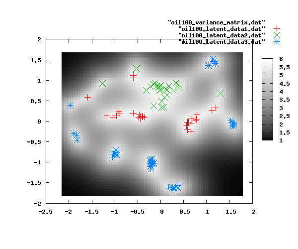
The other files created are
oil100_variance_matrix.dat, which produces the grayscale
map of the log precisions and oil100_latent_data1-3.dat
which are files containing the latent data positions associated with
each label.
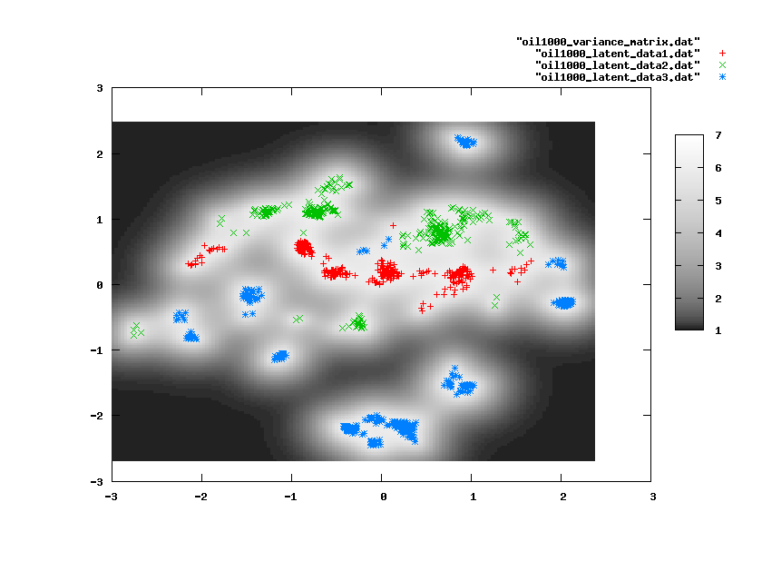
Running the GPLVM for 1000 iterations on all 1000 points of the oil data leads to the visualisation below.
>> gplvmResultsCpp('oil100.model', 'vector')

>>
This will load the results and allow you to move around the latent
space visualising (in the form of a line plotted from the vector) the
nature of the data at each point.
Motion Capture
One popular use of the GPLVM has been in learning of human motion
styles (see Grochow
et al.). Personally, I find this application very
motivating as Motion Capture data is a rare example of high
dimensional data about which humans have a strong intuition. If the
model fails to model `natural motion' it is quite apparant to a human
observer. Therefore, as a second example, we will look at data of this
type. In particular we will consider a data sets containing a walking
man and a further data set containing a horse. To run these demos you
will also need a small MATLAB
mocap toolkit.
BVH Files
To prepare a new bvh file for visualisation you need the MATLAB mocap toolkit and Anton Schwaighofer's SVM light MATLAB interface (you don't need the SVM light software itself).
>> [bvhStruct, channels, frameLength] = bvhReadFile('examples/Swagger.bvh');

>>
This motion capture data was taken from Ohio State University's ACCAD centre.
The motion capture channels contain values for the offset of the root node at each frame. If we don't want to model this motion it can be removed at this stage. Setting the 1st, 3rd and 6th channels to zero removes X and Z position and the rotation in the Y plane.
>> channels(:, [1 3 6]) = zeros(size(channels, 1), 3);
You can now play the data using the command
>> bvhPlayData(bvhStruct, channels, frameLength);
Data in the bvh format consists of angles, this presents a problem when the angle passes through a discontinuity. For example in this data the 'lhumerus' and 'rhumerus' joints rotate through 180 degrees and the channel moves from -180 to +180. This arbitrary difference will seriously effect the results. The fix is to add or subtract 360 as appropriate. In the toolbox provided this is done automatically in the file bvhReadFile.m using the function channelsAngles. This works well for the files we use here, but may not be a sufficient solution for files with more rotation on the joints.
Then channels can be saved for modelling using Schwaighofer's SVM light interface. First we downsample so that things run quickly,
>> channels = channels(1:4:end, :);
Then the data is saved as follows:
>> svmlwrite('examples/swagger.svml',channels)
Before you save you might want to check you haven't messed anything up by playing the data again!
It makes sense to learn
the scale independently for each the channels (particularly since we
have set three of them to zero!), so we now use the gplvm code to
learn the data setting the flag -L true for learning of
scales.
$ ./gplvm -v 3 learn -L true examples/swagger.svml swagger.model
Once learning is complete the results can be visualised in MATLAB using the command
>> mocapResultsCppBvh('swagger.model', 'examples/Swagger.bvh', 'bvh');
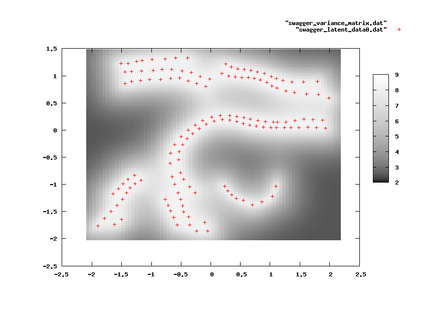
Note that there are breaks in the sequence. These reason for these breaks is as follows. The GPLVM maps from the latent space to the data space with a smooth mapping. This means that points that are nearby in latent space will be nearby in data space. However that does not imply the reverse, i.e. points that are nearby in data space will not necessarily be nearby in latent space. It implies that if points are far apart in data space they will be far apart in latent space which is a slightly different thing. This means that the model is not strongly penalised for breaking the sequence (even if a better solution can be found through not breaking the sequence).
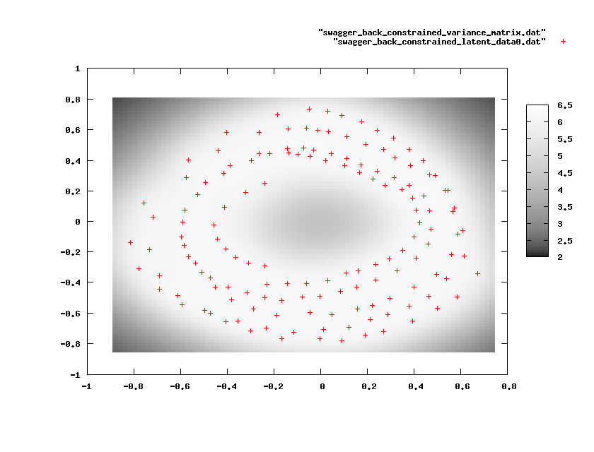
For visualisation you often want points being nearby in data space to be nearby in latent space. For example, most of the recent spectral techniques (including kernel PCA, Isomap, and LLE) try and guarantee this. In recent unpublished work with Joaquin Quinonero Candela, we have shown that this can be achieved in the GPLVM using `back constraints'. We constrain the data in the latent space to be represented by a second reverse-mapping from the data space. For the walking man the show results you can test the back constraints with the command
$ ./gplvm -v 3 learn -L true -c rbf -g 0.0001 examples/swagger.svml swagger_back_constrained.modelThe back constraint here is a kernel mapping with an `RBF' kernel which is specified as having an inverse width of 1e-4. The results can then be seen in MATLAB using
>> mocapResultsCppBvh('swagger_back_constrained.model', 'examples/Swagger.bvh', 'bvh');
It conceptually straightforward to add MAP dynamics in the GP-LVM
latent space by placing a prior that relates the latent points
temporally. There are several ways one could envisage doing this. Wang et al
proposed introducing dynamics through the use of a Gaussian process
mapping across time points. William V. Baxter implemented this
modification to the code and kindly allowed me to make his
modifications available. In the base case adding dynamics associated
with a GP doesn't change things very much: the Gaussian process
mapping is too flexible and doesn't constrain the behaviour of the
model. To solve this problem Wang suggests using a particular prior on
the hyper parameters of the GP-LVM (see pg 58 of his Master's
thesis). This prior is unusual as it is improper, but it is not
the standard uninformative 1/x prior. This approach can be recreated
using the -dh flag when running the code. An alternative
approach of scaling the portion of the likelihood associated with the
dynamics up by a factor has also been suggested. This approach can be
recreated by using the -ds flag.
My own preference is to avoid either of these approaches. A key
motivation of the GP-LVM as a probabilistic model was to design an
approach that avoided difficult to justify scalings and unusual
priors. The basic problem is that if the hyper parameters are
optimised the Gaussian process is too flexible a model for application
modelling the dynamics. However it is also true that a non-linear
model is needed. As an alternative approach we suggest fixing the
hyper parameters. The level of noise can be fixed by suggesting a
signal to noise ratio. This approach has also been implemented in the
code using the -dr flag.
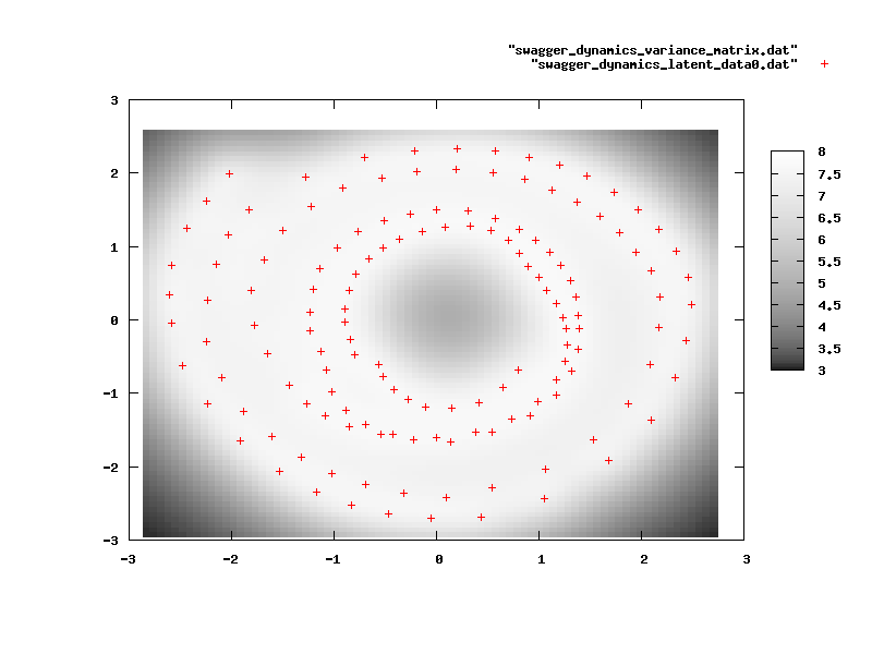
$ ./gplvm -v 3 learn -L true -D rbf -g 0.01 -dr 20 examples/swagger.svml swagger_dynamics.model
where the -M flag sets the parameter associated with
Wang's prior. Here the dynamics GP is given a linear and an RBF
kernel. The results of the visualisation are shown below.
This result can also be loaded into MATLAB and played using the command
>> mocapResultsCppBvh('swagger_dynamics.model', 'examples/Swagger.bvh', 'bvh');