An Efficient Implementation of Gammatone Filters

Syntax

[bm, env, insftp, instf] = gammatone_c(x, fs, cf, hrect) 
 
  x      - input signal
  fs     - sampling frequency (Hz)
  cf     - centre frequency of the filter (Hz)
  hrect  - half-wave rectifying if hrect = 1 (default)
 
  bm     - basilar membrane displacement
  env    - instantaneous envelope
  instp  - instantaneous phase (unwrapped radian)
  instf  - instantaneous frequency (Hz)

Description

An efficient implementation of the 4th order gammatone filter in C as a MEX-function for Matlab. The gammatone filter is widely used in models of the auditory system and is physiologically motivated to mimic the structure of peripheral auditory processing stage. The gammatone function is defined in time domain by its impulse response: Gammatone filter equation

where

is the order of the filter which largely determines the slope of the filter's skirts;

is the bandwidth of the filter and largely determines the duration of the impulse response;

is the amplitude;

is the filter centre frequency; phi

is the phase.

Patterson et al. (1992) show that the impulse response of the gammatone function of order 4 provides an excellent fit to the human auditory filter shapes derived by Patterson and Moore (1986). Glasberg and Moore (1990) have summarised human data on the equivalent rectangular bandwidth (ERB) of the auditory filter with the function:

When the order of the filter is 4, the bandwidth

of the gammatone filter is 1.019 ERB.

A bank of gammatone filters - the gammatone filterbank - is commonly used to simulate the motion of the basilar membrane within the cochlea as a function of time, in which the output of each filter models the frequency response of the basilar membrane at a single place (see Fig. 1). The filterbank is normally defined in such a way that the filter centre frequencies are distributed across frequency in proportion to their bandwidth, known as the ERB scale (Glasberg and Moore, 1990). The ERB scale is approximately logarithmic, on which the filter centre frequencies are equally spaced.

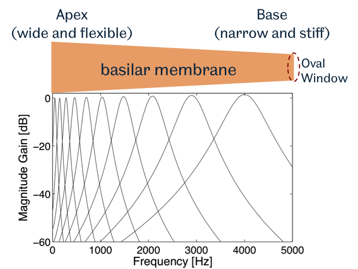
Fig. 1: Frequency responses of a gammatone filterbank with ten filters whose centre frequencies are equally spaced between 50 Hz and 4 kHz on the ERB-rate scale.

Implementation

This gammatone filter implementation is based on Martin Cooke's Ph.D work (Cooke, 1993) using the base-band impulse invariant transformation. For each sample

the signal is first multiplied by a complex exponential $e^{-j2\pi ft}$ at the desired centre frequency, then filtered with a base-band gammatone filter, and finally shifted back to the centre frequency region by multiplying the signal by $e^{j2\pi ft}$ .

The computational cost of the two complex exponentials for every data sample is significant. Our experiment shows that it takes up to 70% of the total computation load. To reduce the computation costs, this implementation transforms the exponential computation into multiplication by rearranging the two complex exponential functions, i.e.,

$e^{-j2\pi ft}=e^{-j2\pi f}e^{-j2\pi f(t-1)}$

where the term $e^{-j2\pi f(t-1)}$ is the exponential calculated for the previous sample at $t$ -1. Therefore only the complex exponential $e^{-j2\pi f}$ for the first sample needs to be computed and the rest can be obtained recursively by multiplication. In practice, the two complex exponential functions are computed using trigonometric functions, i.e., $e^{-j2\pi ft}=\cos(2\pi ft)-j\sin(2\pi ft)$ and $e^{j2\pi ft}=\cos(2\pi ft)+j\sin(2\pi ft)$ .

Informal testing indicates that a gammatone filter of order 4 implemented in this way is 4 times faster than a standard C implementation (Ma et al., 2007) and about 20 times faster than a Matlab implementation. The following example shows a gammatone filter of a centre frequency of 1000 Hz filtering a 3-minute long signal sampled at 16 kHz:

>> tic; bm = gammatone(x, 16000, 1000); toc    %--- Matlab version
Elapsed time is 5.944122 seconds.
>> tic; bm = gammatone_c(x, 16000, 1000); toc  %--- C version
Elapsed time is 0.203346 seconds.

Source code

gammatone_c.c
gammatone_c.m (help file)

Reference

Patterson, R.D. and Moore, B.C.J. (1986) Auditory filters and excitation patterns as representations of frequency resolution. In: Moore, B.C.J. (Eds), Frequency Selectivity in Hearing. Academic Press Ltd., London, pp. 123-177.
Glasberg, B.R. and Moore, B.C.J. (1990) Derivation of auditory filter shapes from notched-noise data. Hearing Research, 47: 103-138.
Patterson, R.D., Robinson, K., Holdsworth, J., McKeown, D., Zhang, C. and Allerhand M. (1992) Complex sounds and auditory images. In: Cazals, Y., Demany, L., Horner, K. (Eds), Auditory physiology and perception, Proc. 9th International Symposium on Hearing. Pergamon, Oxford, pp. 123-177.
Cooke, M. (1993) Modelling auditory processing and organisation. Cambridge University Press
Ma, N., Green, P., Barker, J. and Coy, A. (2007) Exploiting correlogram structure for robust speech recognition with multiple speech sources. Speech Communication, 49 (12): 874-891.